
Trailer Mounted Pump Affinity Laws and Multi-Pump Performance Calculations
Two questions come up constantly on multi-pump and variable-speed deployments and are almost always answered wrong by intuition: how much does a trailer mounted pump‘s curve actually shift when engine speed changes, and how much flow do you actually gain by running two units together instead of one. Both have exact answers derived from pump similarity theory, and both are worked through with real numbers below using this site’s own ZBCY and CHWY product data.
On This Page
- Why This Matters for Variable-Speed and Multi-Pump Deployments
- Deriving the Affinity Laws from Pump Similarity
- Worked Example: Shifting a Curve Across a Speed Range
- Parallel Operation: A Worked Calculation
- Series Operation: A Worked Calculation
- Common Errors in Multi-Pump Curve Math
- Frequently Asked Questions
- A Note on References
Why This Matters for Variable-Speed and Multi-Pump Deployments
A diesel-driven trailer pump running across a variable RPM band, or two units connected in parallel or series, don’t behave according to intuition — they behave according to fixed mathematical relationships derived from pump similarity theory. Guessing at either relationship leads to two specific, common errors covered in this article: assuming a pump throttled down to a lower RPM loses flow in the same proportion it loses head (it doesn’t — the two scale differently), and assuming that running two identical pumps in parallel doubles the flow at a given head (it doesn’t, once the system curve is accounted for). Both relationships are derived below and then applied to real product curves.
Deriving the Affinity Laws from Pump Similarity
The affinity laws follow from a single physical fact: for a given impeller running at different speeds, the flow pattern through the pump remains geometrically similar — velocity triangles at the impeller tip scale in proportion to impeller tip speed, which itself scales directly with rotational speed (u = πDN, where D is impeller diameter and N is rotational speed). Three relationships follow directly from this similarity:
Flow. Volumetric flow through the impeller is proportional to tip speed at a fixed flow area, so flow scales directly with speed:
Head. Euler’s pump equation gives theoretical head as proportional to the product of tip speed and the tangential component of exit velocity (H ∝ u·Cu₂ ÷ g). Since Cu₂ itself scales with tip speed under similar flow conditions, head scales with the square of speed:
Power. Hydraulic power is proportional to the product of flow and head (P ∝ ρgQH). Substituting the flow and head relationships above, power scales with the cube of speed:
These relationships hold with good accuracy for a fixed impeller across a moderate speed range — typically within roughly ±20% of the reference speed, which comfortably covers most diesel trailer pump governor bands. Efficiency is assumed constant across this range in the basic form of the laws; in practice efficiency drifts slightly at the extremes of a wide speed range, which is why manufacturer-published curve families for a given model are the authoritative source when precision matters, with the affinity laws serving as the tool for interpolating between or extrapolating just beyond published curves.
Worked Example: Shifting a Curve Across a Speed Range
The CHWY-16 mixed-flow trailer pump is rated across a 730–980 RPM band, with a published envelope of 1,000–2,300 m³/h flow and 0–20 m head. Taking the 980 RPM condition as the reference point — approximate shutoff head 20 m and approximate maximum flow 2,300 m³/h — the affinity laws predict the curve at 730 RPM as follows. Speed ratio:
Predicted maximum flow at 730 RPM:
Predicted shutoff head at 730 RPM:
This predicted result — a lower-speed curve topping out around 1,700 m³/h and 11 m of head — sits consistently inside the published envelope of 1,000–2,300 m³/h and 0–20 m across the full 730–980 RPM band, confirming the affinity relationship is the right tool for interpolating where in that envelope a specific throttle setting actually lands, rather than assuming the top-of-range figures apply regardless of engine speed. The practical implication: a technician throttling this unit down to conserve fuel on a partial-flow job needs to know they’re not just losing some head — they’re losing head roughly twice as fast (in percentage terms) as they’re losing flow, since head falls with the square of the speed reduction.
Parallel Operation: Curve Addition and a Worked Calculation
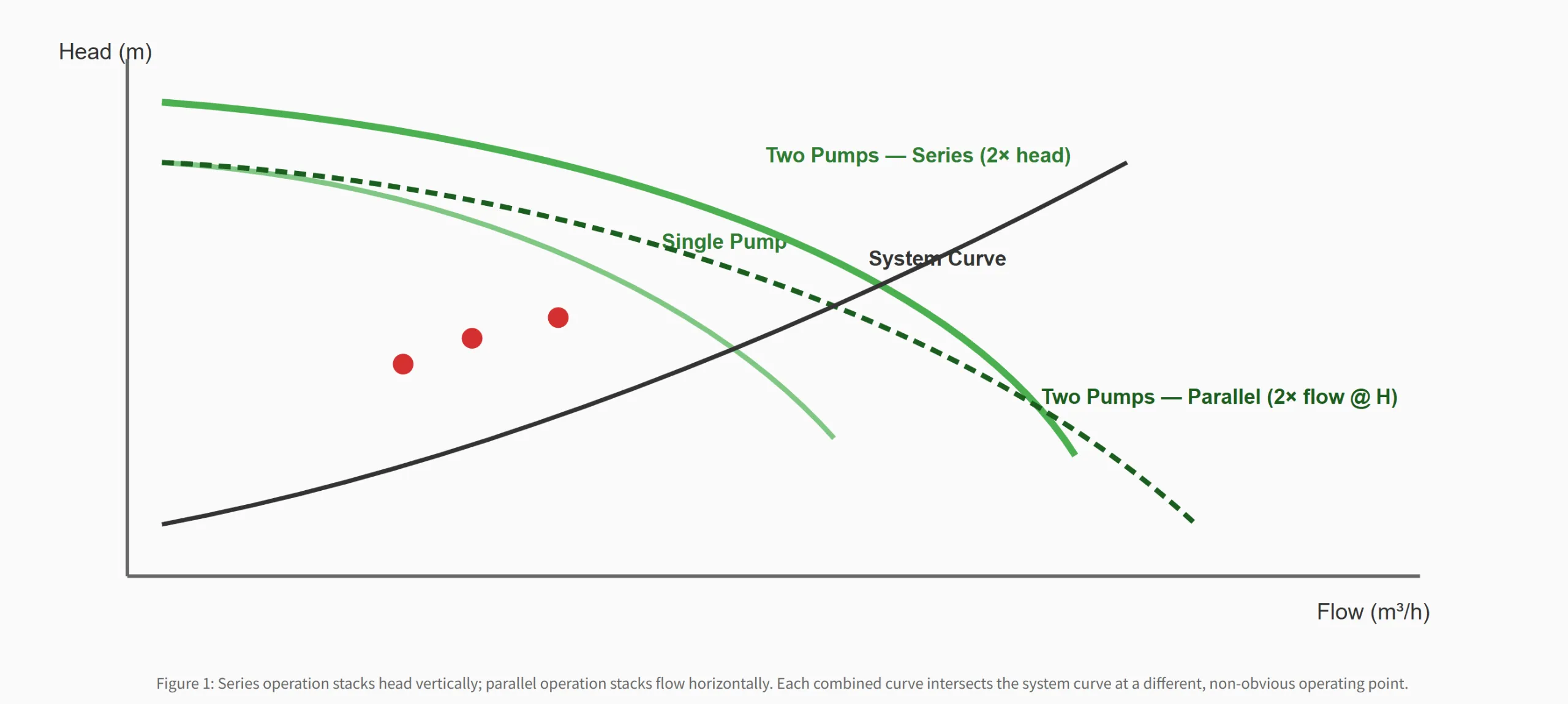
Pumps in parallel add flow at each common head value — the combined curve is built by taking, at every head, the sum of the flow each unit contributes at that head. The combined operating point is then found where this combined curve crosses the system curve, and because the system curve rises with the square of flow, the combined point is never simply double the single-pump flow. Working this through with real numbers: for illustration, the ZBCY200-300-25’s published points (300 m³/h at 0 m head is not the rated condition — its rated point is 300 m³/h at 25 m head; treating 25 m as an approximate shutoff head and 300 m³/h as an approximate zero-head maximum) can be modeled as an idealized parabolic curve for calculation purposes:
Assume a system curve with 8 m of static head and a friction coefficient reflecting the discharge line’s resistance:
Single pump. Setting the pump curve equal to the system curve: 25 − 0.0002778Q² = 8 + 0.00012Q², which gives Q² ≈ 42,735 and Q ≈ 207 m³/h, at a head of roughly 13.1 m.
Two pumps in parallel. Each unit now contributes half the total flow at a given head, so the combined curve is H(Q) = 25 − 0.0002778 × (Q/2)² = 25 − 0.00006945Q². Setting this equal to the system curve: 25 − 0.00006945Q² = 8 + 0.00012Q², giving Q² ≈ 89,738 and Q ≈ 300 m³/h, at a head of roughly 18.8 m.
Two pumps deliver approximately 300 m³/h combined — a 45% increase over the single-pump flow of 207 m³/h, not the 100% increase a naive doubling assumption would predict. The steeper the system curve (longer discharge runs, smaller-diameter hose, more fittings), the smaller this parallel gain becomes, since a rising system curve caps how far right the combined operating point can move regardless of how much additional pump capacity is added.
Series Operation: Curve Addition and a Worked Calculation
Pumps in series add head at each common flow rate instead — used when a single unit’s head capability falls short of what a long bypass run or high static lift demands. Using the same idealized single-pump curve, the combined series curve doubles the head contribution at every flow: H(Q) = 2 × (25 − 0.0002778Q²) = 50 − 0.0005556Q². Set against the same system curve: 50 − 0.0005556Q² = 8 + 0.00012Q², giving Q² ≈ 62,163 and Q ≈ 249 m³/h, at a head of roughly 15.5 m.
Series operation here delivers both more flow (249 vs. 207 m³/h) and reaches a higher head than either pump could sustain alone — useful specifically when the system curve is steep enough that a single unit’s curve doesn’t reach the required head at any usable flow, rather than when more flow alone is the goal, which is what parallel operation is suited to instead.
Common Errors in Multi-Pump Curve Math
Assuming linear doubling in parallel operation. As shown above, the actual gain from adding a second parallel unit depends entirely on how steep the system curve is — a flatter system curve (short, large-diameter discharge) yields a gain closer to true doubling, while a steep system curve (long, narrow discharge, many fittings) yields a much smaller gain, in some cases making a second parallel unit poor value for the job.
Applying affinity laws outside their valid range. The laws hold well within a moderate speed range around the reference point; extrapolating far outside a manufacturer’s tested and published range assumes constant efficiency and identical flow patterns that no longer strictly hold, particularly near the low end of a speed range where internal recirculation and other off-design effects become proportionally larger.
Mismatching pump curves in parallel. Parallel operation assumes both units contribute meaningfully across the shared operating head. Pairing a high-head-capable unit with a lower-head unit in parallel can push the lower-capacity unit toward its shutoff region at the combined operating point, where it contributes little flow while still consuming fuel and wearing its bearings and seals under a low-flow, low-efficiency condition.
Frequently Asked Questions
Q: If I throttle a diesel trailer pump down to 75% of its rated RPM, does it produce 75% of its rated flow?
A: Approximately, yes — flow scales in direct proportion to speed under the affinity laws. Head, however, falls to roughly 56% (0.75²) of its rated value, and power falls to roughly 42% (0.75³) — the three quantities do not scale together.
Q: Why doesn’t running two identical pumps in parallel double my flow rate?
A: Because the system curve’s resistance rises with the square of flow, pushing the combined operating point to a head higher than either pump alone would reach — and at that higher head, each pump individually delivers less flow than it did operating alone. The worked calculation above shows a realistic gain closer to 45% for a specific system curve, not 100%.
Q: When should I use series operation instead of parallel?
A: When the required head exceeds what a single unit’s curve can reach at any usable flow — series operation is a head-boosting configuration. Parallel operation is a flow-boosting configuration for cases where head requirements are already within a single unit’s range but more flow is needed.
Q: How accurate are the affinity laws in practice?
A: Very accurate for flow and head within a moderate range of the reference speed — errors are typically small enough for practical field planning. Accuracy degrades toward the edges of a wide speed range because efficiency isn’t perfectly constant across the whole band, which is why manufacturer-published curve families remain the reference of record for critical sizing decisions.
A Note on References
The affinity laws and multi-pump combination rules used in this article are standard centrifugal pump theory, most authoritatively documented in the Hydraulic Institute’s ANSI/HI 1.3 (Rotodynamic Centrifugal Pumps for Design and Application), which covers both single-pump performance prediction and the accepted method for combining pump curves in series and parallel configurations. Pump Handbook by Karassik, Messina, Cooper, and Heald remains the standard academic and industry reference for the underlying similarity theory and Euler’s pump equation derivation referenced above.
If you’re planning a multi-pump deployment and want the combined operating point calculated against your actual system curve rather than an assumed one, contact the CannaSpring engineering support team with your pump models, arrangement, and discharge line specifications.